Download TCGA data
Download MAF file using TCGABiolinks
MAFDash provides a wrapper function that tries to simplify retrieving data using TCGAbiolinks. Valid project codes can be viewed by running TCGAbiolinks::getGDCprojects() and checking the “tumor” column.
library(MAFDash)
library(TCGAbiolinks)
library(maftools)
tcga_code <- c("ACC","UVM")
#inputFolderPath <- paste0(tempdir()) ## This folder will be created if it doesn't exist
caller = "mutect2"
title_label = paste0("TCGA-",tcga_code)
maf_files <- getMAFdataTCGA(tcga_code,variant_caller = caller)
#>
|
| | 0%
|
| | 1%
|
|= | 1%
|
|= | 2%
|
|== | 2%
|
|== | 3%
|
|=== | 4%
|
|=== | 5%
|
|==== | 5%
|
|==== | 6%
|
|===== | 7%
|
|===== | 8%
|
|====== | 8%
|
|====== | 9%
|
|======= | 9%
|
|======= | 10%
|
|======= | 11%
|
|======== | 11%
|
|======== | 12%
|
|========= | 12%
|
|========= | 13%
|
|========== | 14%
|
|========== | 15%
|
|=========== | 15%
|
|=========== | 16%
|
|============ | 17%
|
|============= | 18%
|
|============= | 19%
|
|============== | 20%
|
|=============== | 21%
|
|=============== | 22%
|
|================ | 22%
|
|================ | 23%
|
|================= | 24%
|
|================= | 25%
|
|================== | 25%
|
|================== | 26%
|
|=================== | 27%
|
|=================== | 28%
|
|==================== | 28%
|
|==================== | 29%
|
|===================== | 30%
|
|====================== | 31%
|
|====================== | 32%
|
|======================= | 33%
|
|======================== | 34%
|
|======================== | 35%
|
|========================= | 35%
|
|========================= | 36%
|
|========================== | 37%
|
|========================== | 38%
|
|=========================== | 38%
|
|=========================== | 39%
|
|============================ | 39%
|
|============================ | 40%
|
|============================= | 41%
|
|============================= | 42%
|
|============================== | 43%
|
|=============================== | 44%
|
|================================ | 45%
|
|================================ | 46%
|
|================================= | 47%
|
|================================= | 48%
|
|================================== | 48%
|
|================================== | 49%
|
|=================================== | 49%
|
|=================================== | 50%
|
|=================================== | 51%
|
|==================================== | 51%
|
|==================================== | 52%
|
|===================================== | 52%
|
|===================================== | 53%
|
|====================================== | 54%
|
|====================================== | 55%
|
|======================================= | 56%
|
|======================================== | 57%
|
|========================================= | 58%
|
|========================================= | 59%
|
|========================================== | 60%
|
|=========================================== | 61%
|
|=========================================== | 62%
|
|============================================ | 62%
|
|============================================ | 63%
|
|============================================ | 64%
|
|============================================= | 64%
|
|============================================= | 65%
|
|============================================== | 65%
|
|============================================== | 66%
|
|=============================================== | 67%
|
|=============================================== | 68%
|
|================================================ | 68%
|
|================================================ | 69%
|
|================================================= | 69%
|
|================================================= | 70%
|
|================================================= | 71%
|
|================================================== | 71%
|
|================================================== | 72%
|
|=================================================== | 73%
|
|==================================================== | 74%
|
|==================================================== | 75%
|
|===================================================== | 76%
|
|====================================================== | 77%
|
|====================================================== | 78%
|
|======================================================= | 78%
|
|======================================================= | 79%
|
|======================================================== | 79%
|
|======================================================== | 80%
|
|======================================================== | 81%
|
|========================================================= | 81%
|
|========================================================= | 82%
|
|========================================================== | 82%
|
|========================================================== | 83%
|
|=========================================================== | 84%
|
|=========================================================== | 85%
|
|============================================================ | 86%
|
|============================================================= | 87%
|
|============================================================== | 88%
|
|============================================================== | 89%
|
|=============================================================== | 89%
|
|=============================================================== | 90%
|
|=============================================================== | 91%
|
|================================================================ | 91%
|
|================================================================ | 92%
|
|================================================================= | 92%
|
|================================================================= | 93%
|
|================================================================== | 94%
|
|================================================================== | 95%
|
|=================================================================== | 95%
|
|=================================================================== | 96%
|
|==================================================================== | 97%
|
|===================================================================== | 98%
|
|===================================================================== | 99%
|
|======================================================================| 99%
|
|======================================================================| 100%
#>
[1mindexed
[0m
[32m2.79kB
[0m in
[36m 0s
[0m,
[32m278.82MB/s
[0m
[1mindexed
[0m
[32m1.00TB
[0m in
[36m 0s
[0m,
[32m12.40TB/s
[0m
|
| | 0%
|
|= | 2%
|
|== | 3%
|
|=== | 5%
|
|==== | 6%
|
|===== | 8%
|
|======= | 9%
|
|======== | 11%
|
|========= | 13%
|
|========== | 14%
|
|=========== | 16%
|
|============ | 17%
|
|============= | 19%
|
|============== | 21%
|
|=============== | 22%
|
|================= | 24%
|
|================== | 25%
|
|=================== | 27%
|
|==================== | 28%
|
|===================== | 30%
|
|====================== | 32%
|
|======================= | 33%
|
|======================== | 35%
|
|========================= | 36%
|
|=========================== | 38%
|
|============================ | 40%
|
|============================= | 41%
|
|============================== | 43%
|
|=============================== | 44%
|
|================================ | 46%
|
|================================= | 47%
|
|================================== | 49%
|
|=================================== | 51%
|
|===================================== | 52%
|
|====================================== | 54%
|
|======================================= | 55%
|
|======================================== | 57%
|
|========================================= | 58%
|
|========================================== | 60%
|
|=========================================== | 62%
|
|============================================ | 63%
|
|============================================= | 65%
|
|============================================== | 66%
|
|================================================ | 68%
|
|================================================= | 70%
|
|================================================== | 71%
|
|=================================================== | 73%
|
|==================================================== | 74%
|
|===================================================== | 76%
|
|====================================================== | 77%
|
|======================================================= | 79%
|
|======================================================== | 81%
|
|========================================================== | 82%
|
|=========================================================== | 84%
|
|============================================================ | 85%
|
|============================================================= | 87%
|
|============================================================== | 88%
|
|=============================================================== | 90%
|
|================================================================ | 91%
|
|================================================================= | 93%
|
|================================================================== | 95%
|
|=================================================================== | 96%
|
|==================================================================== | 98%
|
|======================================================================| 99%
|
|======================================================================| 100%
#>
[1mindexed
[0m
[32m2.44kB
[0m in
[36m 0s
[0m,
[32m301.50MB/s
[0m
[1mindexed
[0m
[32m1.00TB
[0m in
[36m 0s
[0m,
[32m21.99TB/s
[0m
Download clinical data using TCGABiolinks
# tcga_clinical <- getTCGAClinicalAnnotation#TCGAbiolinks::GDCquery_clinic(project = paste0("TCGA-",tcga_code), type = "clinical")
# tcga_clinical$Tumor_Sample_Barcode <- tcga_clinical$submitter_id
#defaultW <- getOption("warn")
#options(warn = -1)
tcga_clinical<-getTCGAClinicalAnnotation(cancerCodes = tcga_code)
#options(warn = defaultW)
Make a customized oncoplot
Filter data
The filterMAF function can be used to filter the MAF data in various ways. Importantly, by default, it will remove commonly occurring mutations that are often considered to be false position ( FLAG genes )
Add clinical data
The easiest way to add clinical annotations to the oncoplot is to add clinical data to the clinical.data slot of a MAF object before passing it to the generateOncoplot() function.
MAFDash also provides a function that defines reasonable colors for some common clinical annotations provided with TCGA datasets.
filtered_maf <- read.maf(filtered_mafdata, clinicalData = tcga_clinical$annodata,verbose = FALSE)
annotation_colors <- getTCGAClinicalColors(ageRange = range(tcga_clinical$annodata$age_at_diagnosis, na.rm=T))
Make an annotated oncoplot
The add_clinical_annotations argument can be:
- A boolean indicating whether or not to add annotations built from the
clinical.dataslot of theMAFobject. Columns with all missing values are ignored. Maximum number of annotations plotted is 10 (first 10 non-empty columns ofclinical.data) - A character vector of column names provided as clinical data
custom_onco <- generateOncoPlot(filtered_maf,
                                add_clinical_annotations = names(annotation_colors),
                                clin_data_colors = annotation_colors)
custom_onco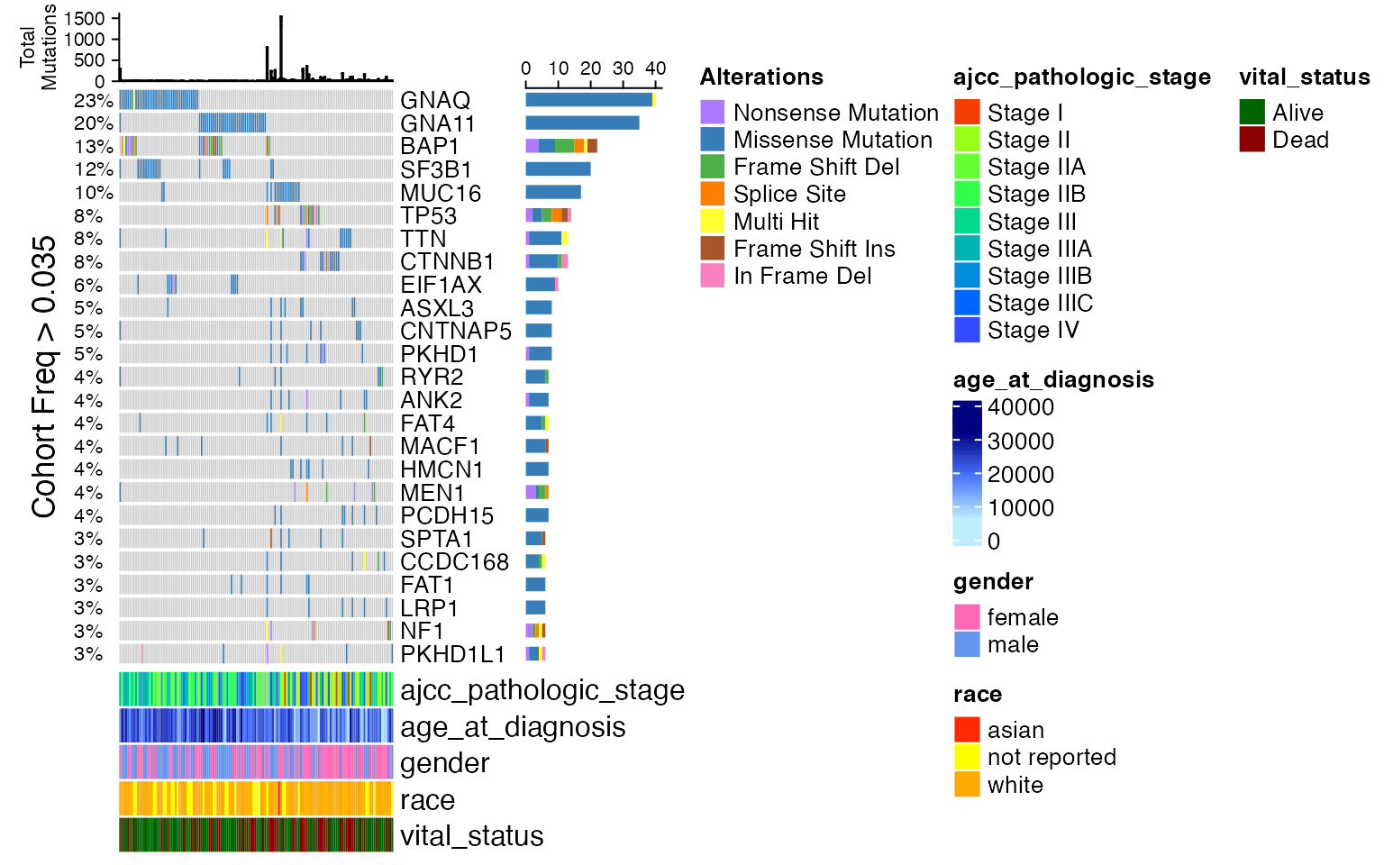
Make some other figures
TCGA Comparison
A lot of maftools’s plots are base graphics, so they’re drawn to a device and not returned. But we can simply save them to a file and provide the file path.
tcgaComparePlot<-generateTCGAComparePlot(maf = filtered_maf, cohortName = "test")
tcgaComparePlot$tcga_compare_plot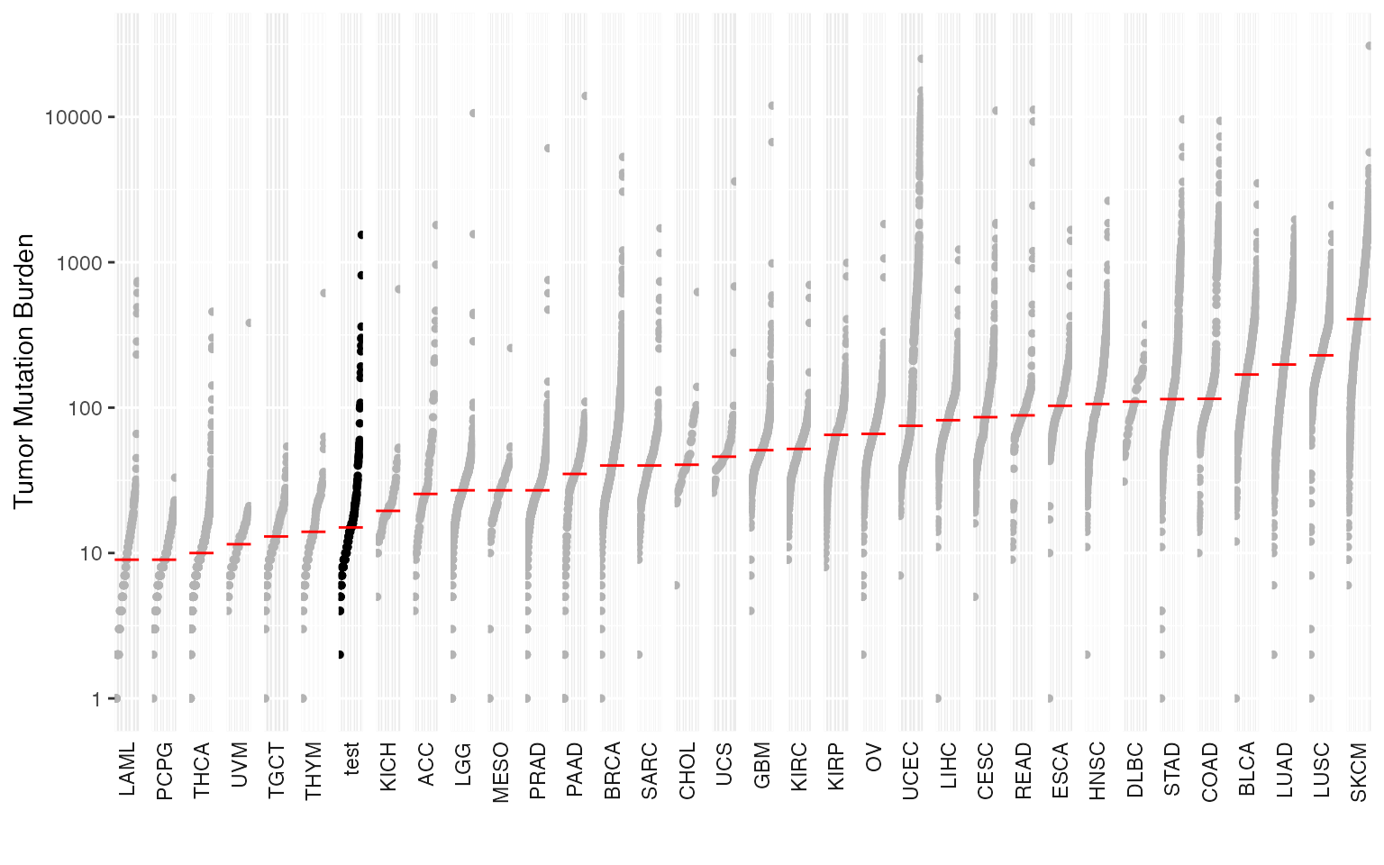
Chord Diagram of mutation co-occurrence
This function is built on top of maftools’s somaticInteractions() function. It’s just a different way of visualizing co-occurence or mutual exclusivity between genes.
#ribbonplot_file <- file.path(getwd(),"ribbon.pdf")
generateRibbonPlot(filtered_maf,save_name = NULL)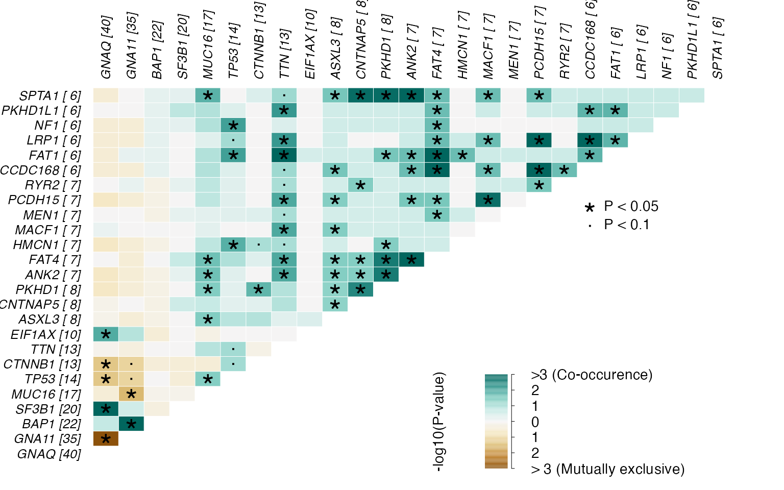
###Plot similarity to COSMIC signatures The function generateCOSMICMutSigSimHeatmap computes the cosine similarity of each individual signature against each COSMIC signature. The COSMIC signatures are also annotated using the etiologies behind the mutational signatures that were identified by analyzing thousands of whole-genome sequencing samples from TCGA. A crawler script was used to scrape the etiologies in the “Acceptance criteria” section of each signature page from COSMIC database v3.2.
library(ComplexHeatmap)
val<-generateCOSMICMutSigSimHeatmap(filtered_maf)
#> -Extracting 5' and 3' adjacent bases
#> -Extracting +/- 20bp around mutated bases for background C>T estimation
#> -Estimating APOBEC enrichment scores
#> --Performing one-way Fisher's test for APOBEC enrichment
#> ---APOBEC related mutations are enriched in  17.059 % of samples (APOBEC enrichment score > 2 ;  29  of  170  samples)
#> -Creating mutation matrix
#> --matrix of dimension 172x96
draw(val)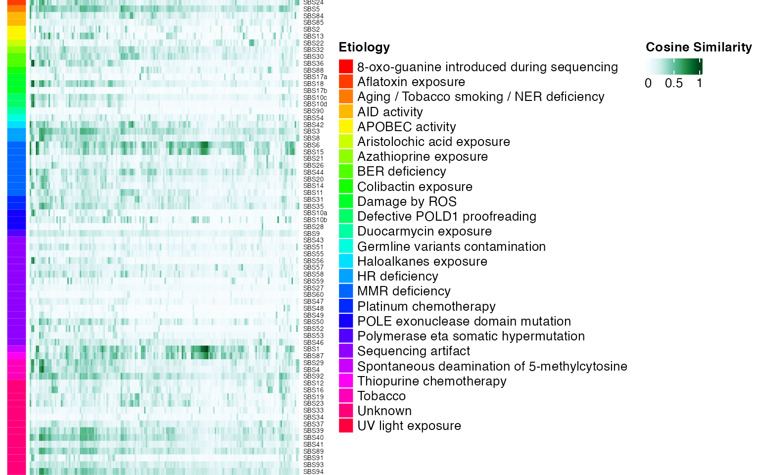
Render the dashboard
customplotlist <- list("summary_plot"=T,
                       "burden"=T,
                       "TCGA Comparison"=tcgaComparePlot$tcga_compare_plot,
                       "oncoplot"=T,
                       "Annotated Oncoplot"=custom_onco
                       )

## Filename to output to; if output directory doesn't exist, it will be created
html_filename=file.path(paste0(tempdir(),"/TCGA-UVM.custom.mafdash.html"))

## Render dashboard
getMAFDashboard(MAFfilePath = filtered_maf,
                plotList = customplotlist,
                outputFileName = html_filename,
                outputFileTitle = "Customized Dashboard")
Output
The output can be seen here.